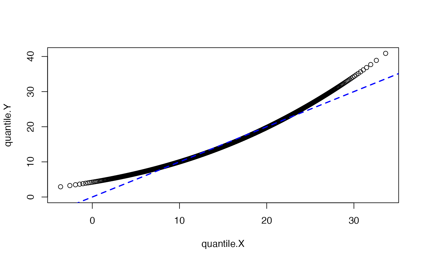
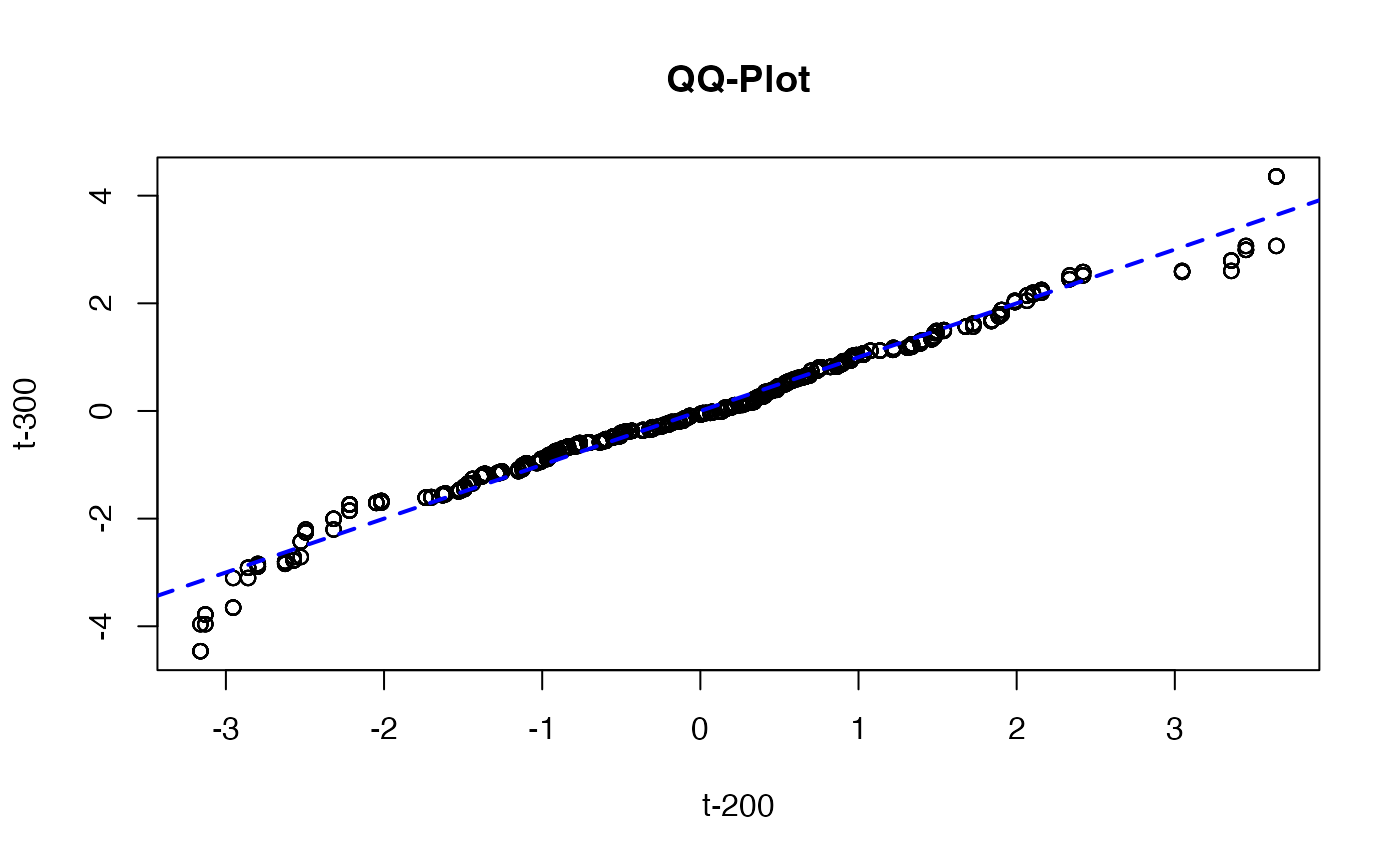
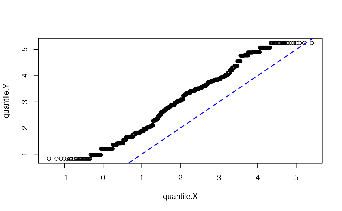
Quantile-quantile plots are used to compare a "theoretical" or empirical distribution to a reference distribution. They can also compare the quantiles of two reference distributions.
qqplot(x, y, npoints = 3000, idline = TRUE, plot = TRUE, ...)Arguments
- x
distr6object or numeric vector.- y
distr6object or numeric vector.- npoints
number of evaluation points.
- idline
logical; if TRUE (default), the line \(y = x\) is plotted
- plot
logical; if TRUE (default), figures are displayed in the plot window; otherwise a data.table::data.table of points and calculated values is returned.
- ...
graphical parameters.
Details
If x or y are given as numeric vectors then they are first passed to the
Empirical distribution. The Empirical distribution is a discrete distribution so quantiles
are equivalent to the the Type 1 method in quantile.
See also
plot.Distribution for plotting a distr6 object.


